Outputs
This page describes generated outputs (CSV tables, LUTs, corrected fluxes, and diagnostic figures).
Output folder structure
Outputs are written to the folder configured by output_path. In the repository example run, outputs are
available under:
examples/output/
Filenames include a site name and run metadata (gas, workflow, time window, timestamp).
CSV outputs
The following CSV files are typically produced.
Cut-off frequency LUT
4_LUT_cof__<site>__<gas>__<mode>__... .csv
This table stores the cut-off frequency look-up table used by the workflow. In the example run it contains one row per wind-direction / wind-speed class (depending on configuration), with columns such as:
wd_mean,wd_max,unc_wdclassws_mean,ws_maxcof_L,cof_G: cut-off frequencies for the Lorentzian / Gaussian transfer-function fitsfn_L,fn_G: normalized frequenciesunc_L_tf,unc_G_tf: transfer-function-related uncertainty on the fitted cut-off frequencies (per class)
Mean (co)spectra
4_mean_cosp__<site>__<gas>__<mode>__... .csv
This table stores averaged (co)spectra per class and frequency bin. It is primarily used for diagnostics and plotting.
Correction factor LUT
5_LUT_CF__<site>__<gas>__<mode>__... .csv
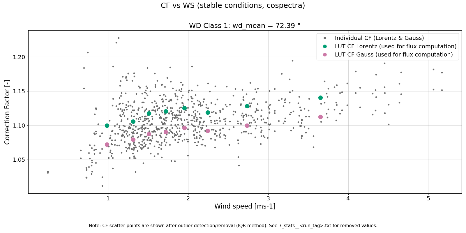
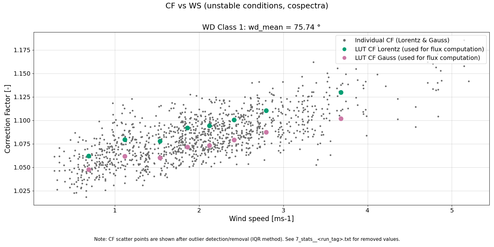
This table stores correction factors (stable/unstable) aggregated by class. In the example output, the file
contains two blocks (unstable then stable), each providing (among others):
wd_mean,ws_meanCF_L,CF_G: correction factors for Lorentzian / Gaussian approachesunc_L_tf,unc_G_tf: transfer-function-related uncertainty component (computed as the maximum deviation from the central CF value “M”)unc_L_sd,unc_G_sd: within-class spread of CF values (standard deviation computed after outlier removal)
Note: total uncertainties are not written to the output anymore; users can recompute them as needed from the component uncertainties.
Corrected flux output
6_flux_out__<site>__<gas>__<mode>__... .csv
This is the main half-hourly output time series. In the example output it includes:
Timestampmeteorological descriptors used for classification (e.g.
wind_speed (m s-1),wind_dir (deg),(z-d)/L (-))original flux columns (e.g.
Fc (µmol m-2 s-1),FcEP (µmol m-2 s-1))corrected fluxes (e.g.
FCcorL,FCcorG)correction factors applied (
CF_L,CF_G)
Diagnostic figures
When plotting is enabled, FREQCOR generates diagnostic figures to help evaluate selection steps, transfer function fitting, LUT construction, and correction-factor behavior.
The following figures are shown from the example BE-Lon CO2 cospectral run.
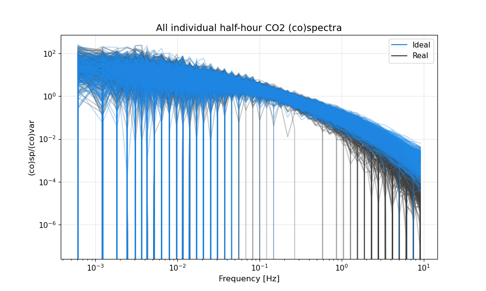
Individual (co)spectra
This figure shows individual (co)spectra contributing to the computation (after initial selection), used to evaluate variability and potential outliers.
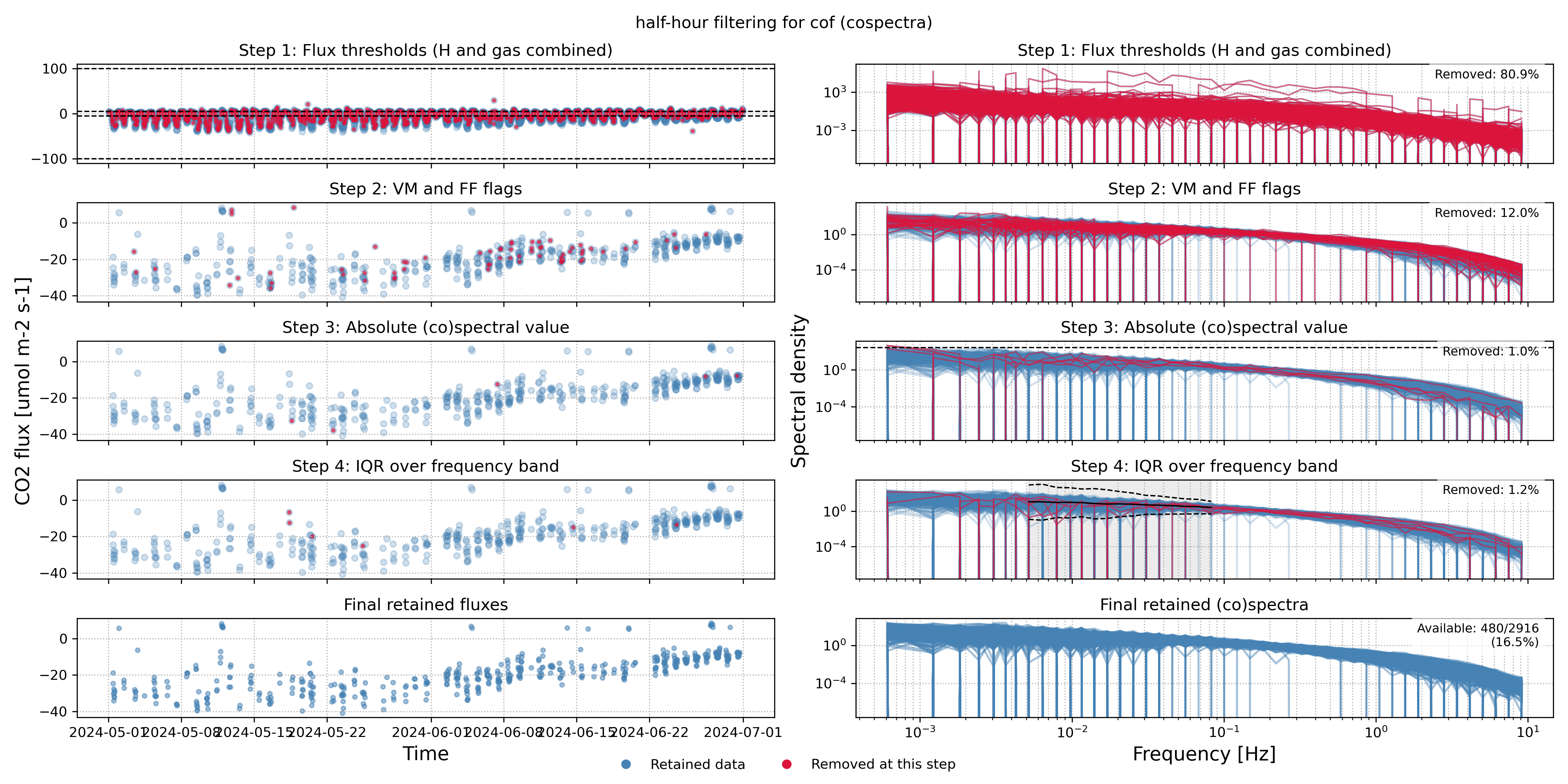
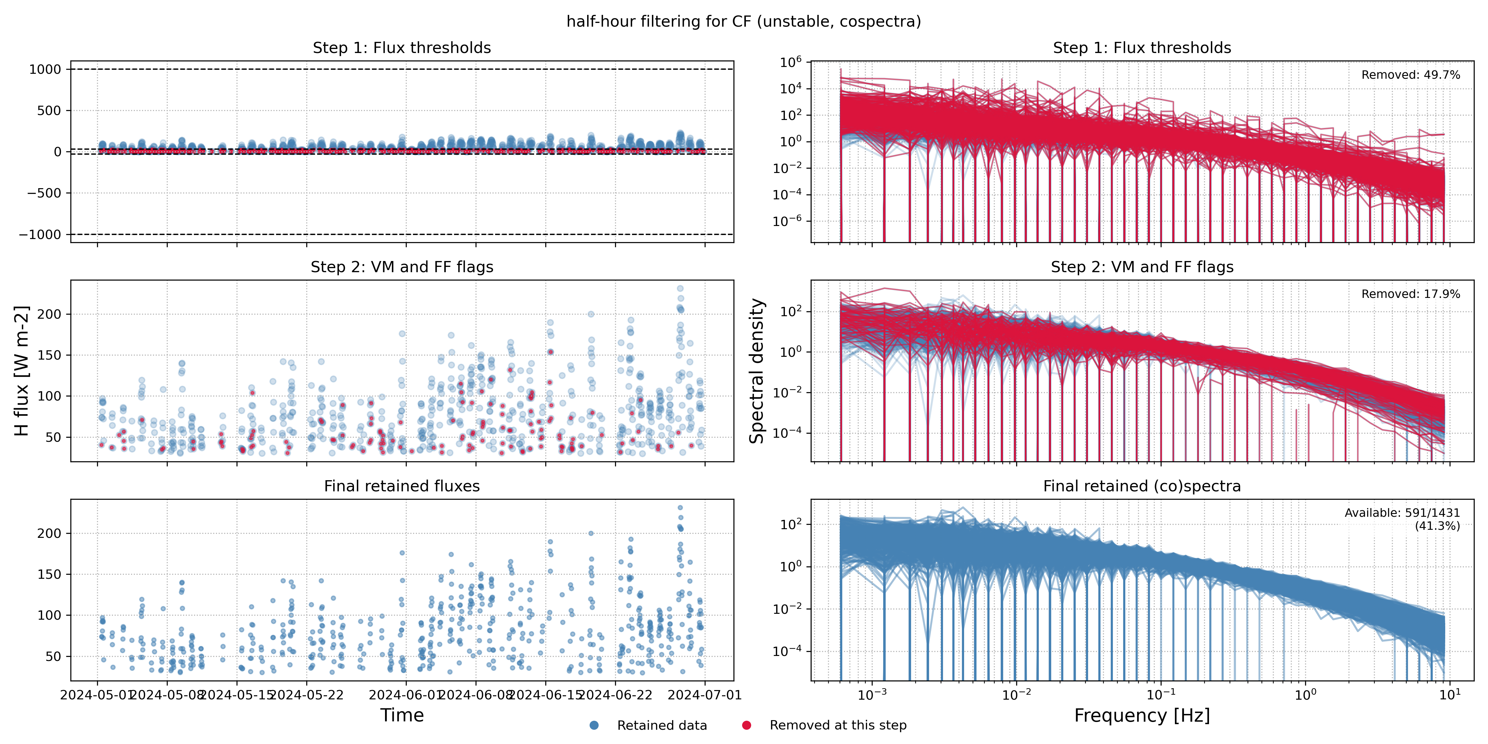
Filtering diagnostics
These figures illustrate how data were filtered when estimating cut-off frequencies and correction factors.
Mean transfer functions and mean cospectra
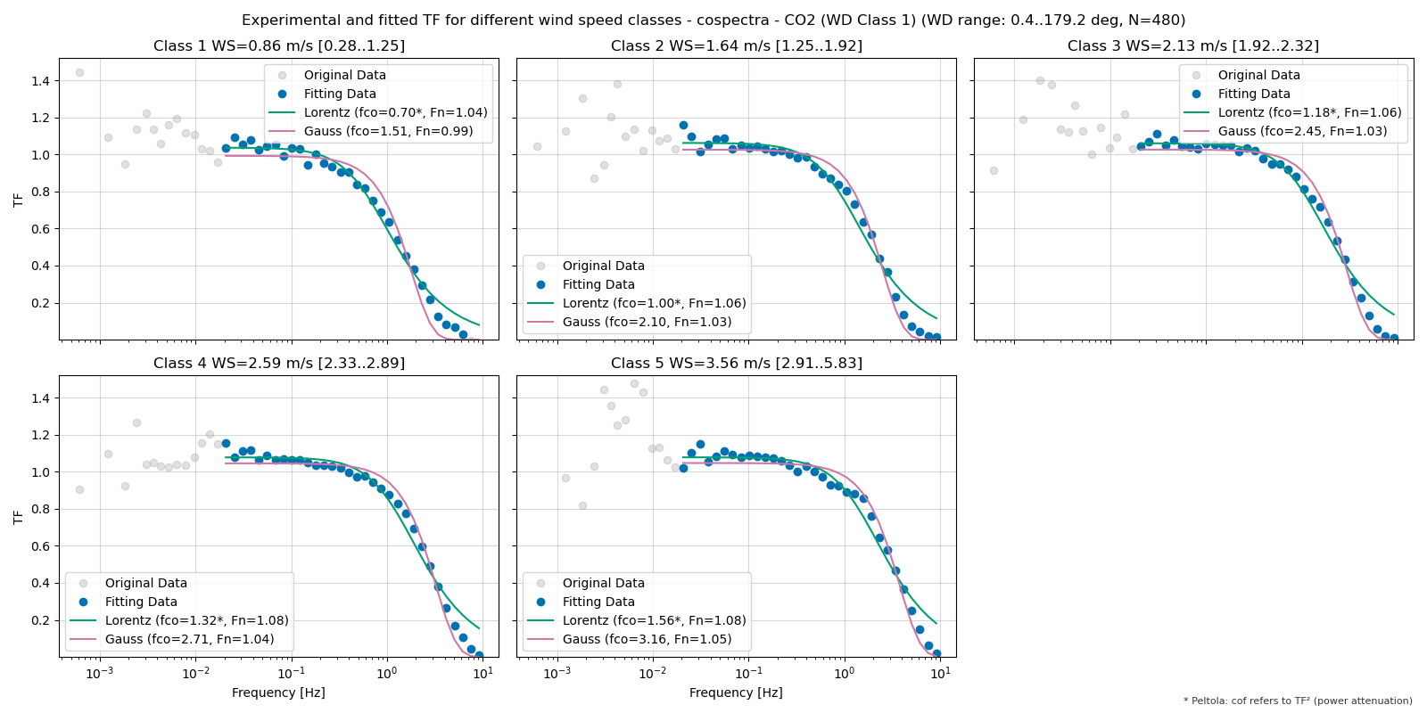
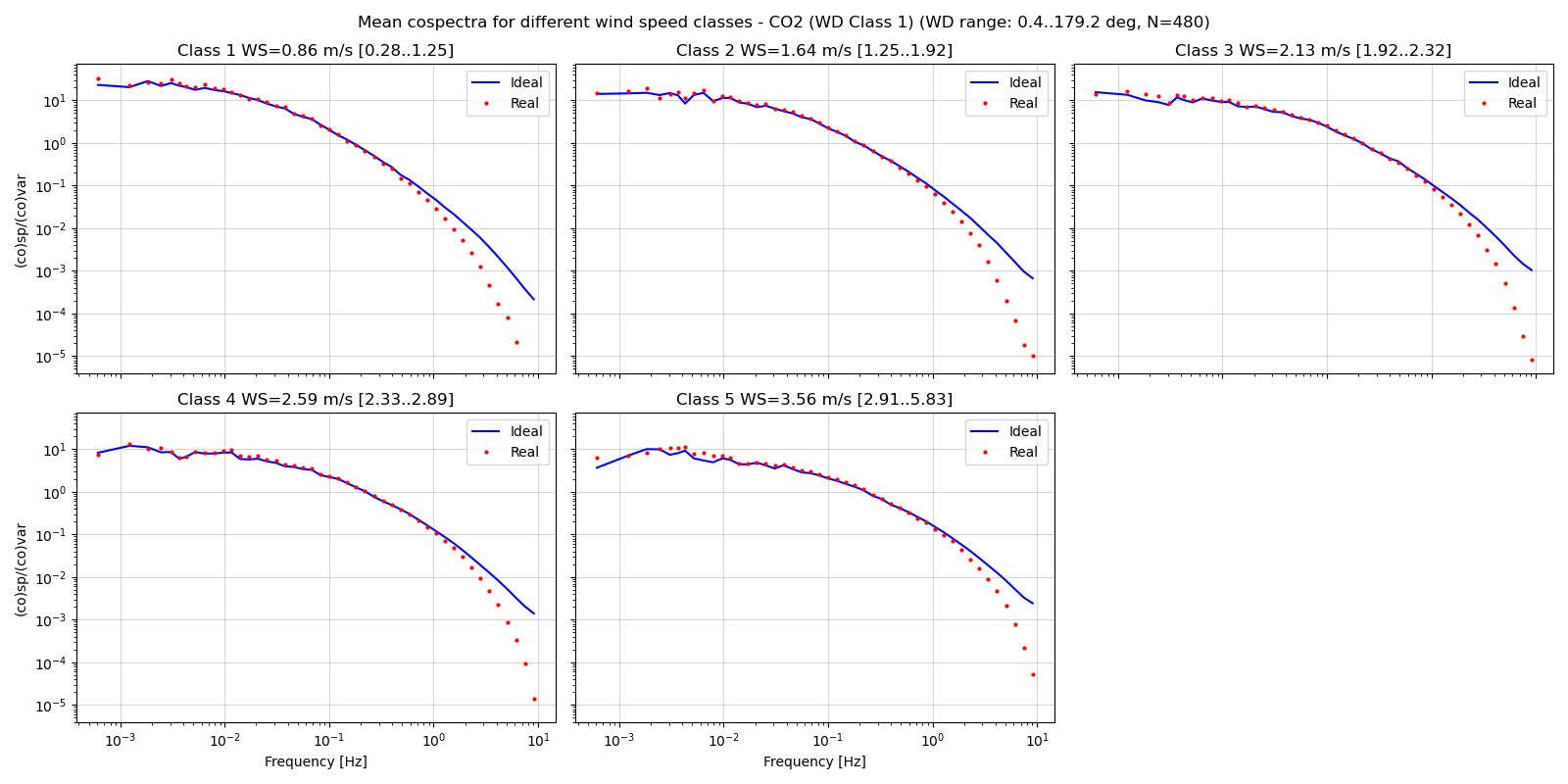
These figures summarize transfer functions and (co)spectra averaged over classes.
Correction factors
These figures show the correction factors as a function of wind speed for stable and unstable regimes.